A recursive function is a function that calls itself.
We already saw an example of recursive program when we did the Greatest common divisor algorithm. Another typical example is the factorial of a number. The factorial of a number n is the product of 1*2..(n-1)*n. And it is written as n!. Mathematically we can see that this definition can also be described as: n!=n*(n-1)!. Here you can see that the function definition uses itself. To be able to do this we need some initial values, or else we could repeat it infinitely. For the factorial function the initial value is that 0! = 1. This base case is very important because it will allow the program to stop.
With this two definitions we can start programming our function.
       function factorial(n) {
	  if (n == 0) {
		return 1
	  }
   	  return n * factorial(n - 1)
        }

        var num = input()
        output(factorial(num))
Although some times the transformation between the recursive definition of a problem and the program itself might look easy, it is not always the best solution. A clear example is the Fibonacci numbers problem . As you can read in the wikipedia article, by definition, the first two numbers in the Fibonacci sequence are either 1 and 1, or 0 and 1, depending on the chosen starting point of the sequence, and each subsequent number is the sum of the previous two.
Translated into mathematical notation we get that F0=1, F1=1 and Fn=Fn-1+Fn-2 .
And translating this into a program we have:
        function Fibonacci(n) {
	   if (n == 0 || n == 1) {
		return 1
	   }
	   return Fibonacci(n - 1) + Fibonacci(n - 2)
        }

        var num = input()
        output(Fibonacci(num))
The main problem with this code is that we compute many times the same values. If we modify a little to see how many operations we use we can understand better what is happening:
        function Fibonacci(n) {
	       output("Computing Fibonacci of " + n)
	       calls++
	       if (n == 0 || n == 1) {
		    return 1
	        }
	        return Fibonacci(n - 1) + Fibonacci(n - 2)
         }

         var calls = 0
         var num = input()
         output(Fibonacci(num))
         output(calls)
If we check how many operations we need to compute the 10th number of Fibonacci the answer is 177 and the 11th requires 287 operations. If we do a table we will see the growth between consecutive numbers.
| n | Value | Calls |
|---|---|---|
| 10 | 89 | 177 |
| 11 | 144 | 287 |
| 12 | 233 | 465 |
| 13 | 377 | 753 |
Here we can notice 2 things. First of all the numbers grow in an exponential way (almost double every time). Second if we look closer each number (in the calls column) is the sum of the previous two plus 1. This comes from the fact that to compute the n-th fibonacci number we need to compute also the previous 2, and we have an extra call to sum those results.
But how can we make our program more efficient? This will be seen in the next part called Memoization.
Memoization is a technique in computer science where you store values you have already calculated to be able to access them in future queries. In this way you don't need to compute them twice.
In the previous example we computed Fibonacci numbers and we saw we did an exponential number of operations. If we apply memoization, this number can become linear. This means that a small increase of the input will require a small increase in the operations used. The program will look like this.
       function Fibonacci(n) {
	     if (n == 0 || n == 1) {
		  return 1
	     }
	     if (values[n] != undefined) {
		  return values[n]
	     }
	     return values[n] = Fibonacci(n - 1) + Fibonacci(n - 2)
       }

       var values = []
       var num = input()
       repeat (num + 1) {
	     values.push()
       }
       output(Fibonacci(num))
As you can see the array values will store all the Fibonacci numbers computed until that point. This algorithm is much faster than the previous one. You can try to compute the number of operations it does and study it's growth as in the previous example!
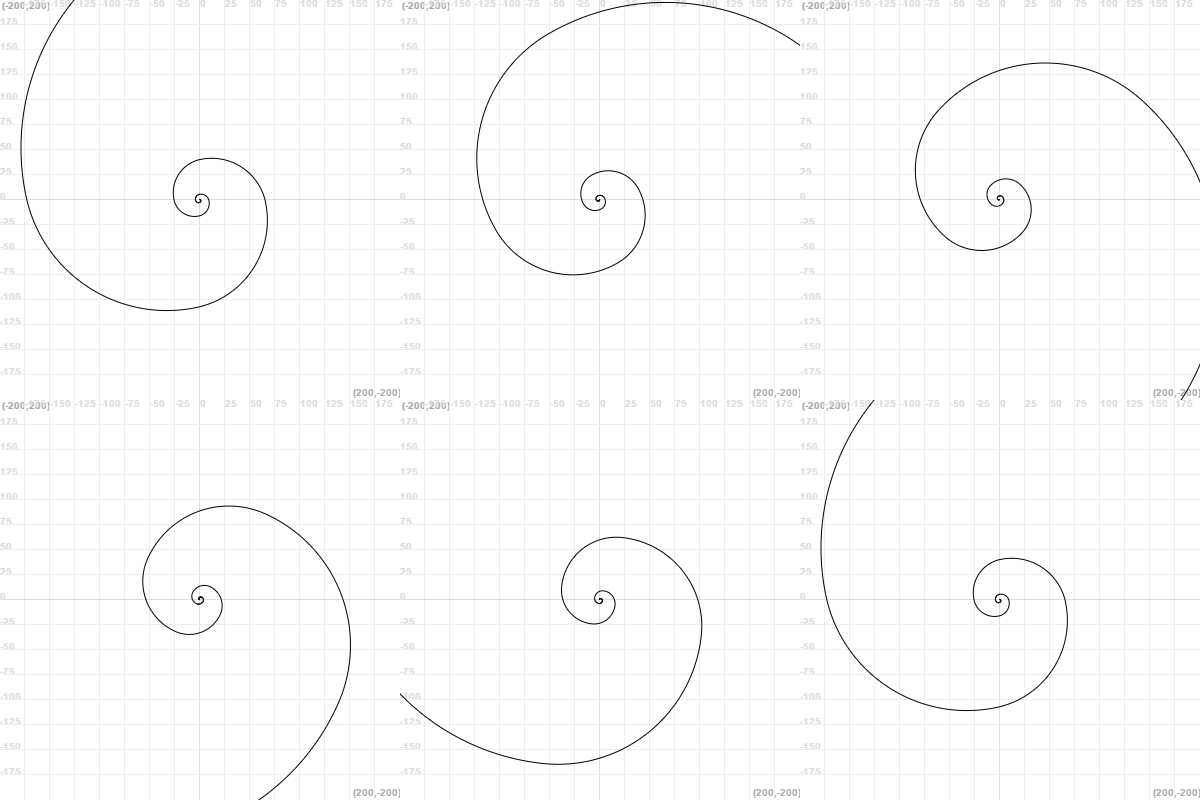
There are many projects that can be done with a little knowledge on recursive programming. Here are some codes of example. Try reading them and change whatever you want to explore! Good Luck!
Fibonacci spiral (using recursion as a substitute of an iterative process)
      function fibonacci(a, b, limit) {
	if (limit != 0) {
		arc(b, 90, true)
		fibonacci(b, a + b, limit - 1)
	}
      }

     repeat (30) {
	goToCenter()
	clean()
	fibonacci(1, 1, 12)
	turnRight(12)
	snapshot()
      }
      animateLayers(0.1)
Plant (based on Lindenmayer Fractals)
        function plant(size, angle) {
	     if (size < 1) {
		return
	     }
	     turnRight(angle)
	     forward(size)
	     repeat (4) {
		plant(size - 9, getRandomNumber(160) - 80)
	    }
	    forward(-size)
	    turnLeft(angle)
        }

        goToCenter()
        turnLeft(90)
        plant(50, 0)
Koch Fractal (from our Merry Everything article)
      // Recursive Koch fractal function
       function koch_snowflake_side(length, depth) {
	     if (depth == 0) {
		forward(length)
		return
	      }
	      koch_snowflake_side(length / 3, depth - 1)
	      turnRight(60)
	      koch_snowflake_side(length / 3, depth - 1)
	      turnLeft(120)
	      koch_snowflake_side(length / 3, depth - 1)
	      turnRight(60)
	      koch_snowflake_side(length / 3, depth - 1)
        }

       repeat (3) {
	      koch_snowflake_side(180, 4)
	      turnLeft(120)
       }
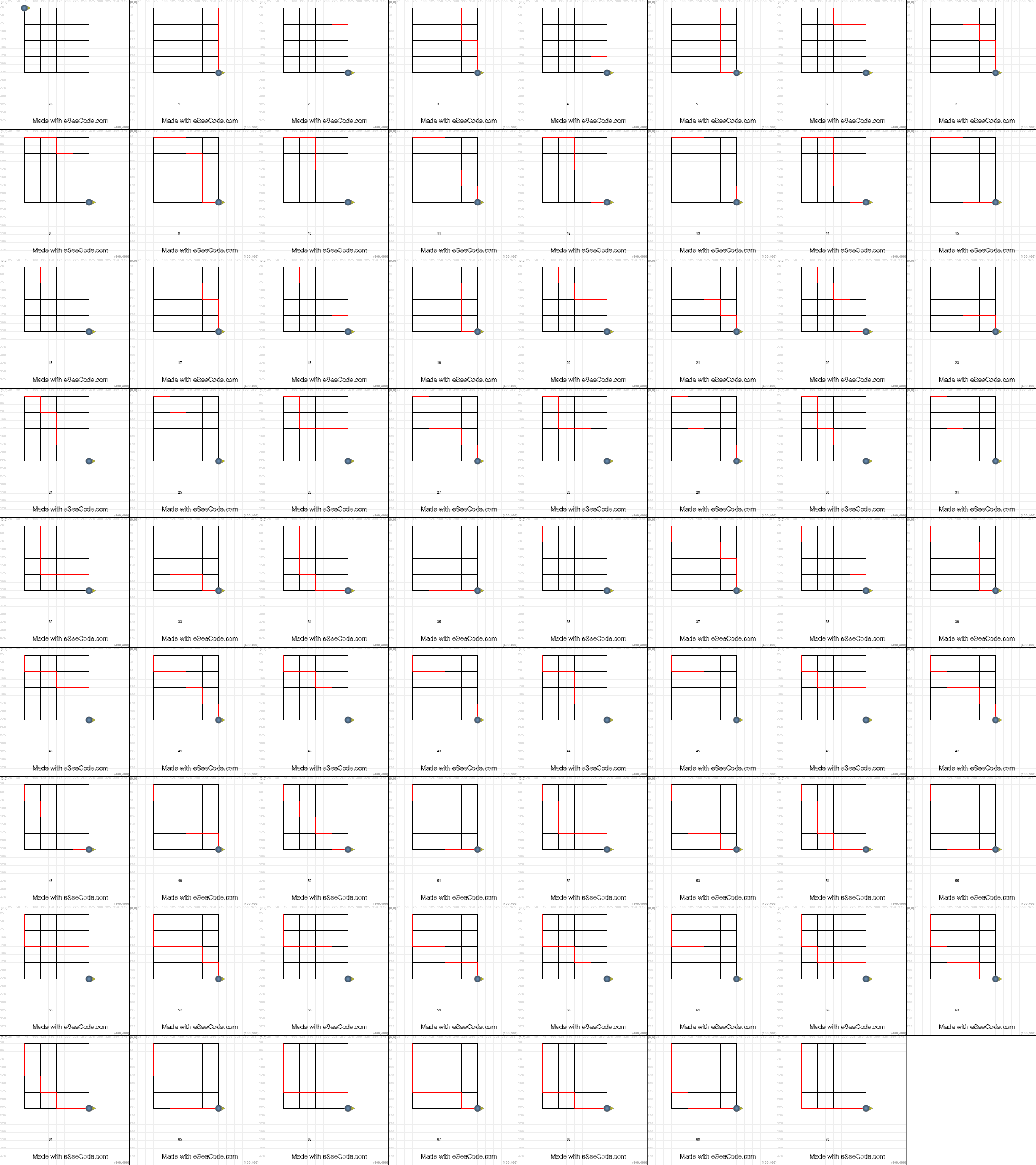
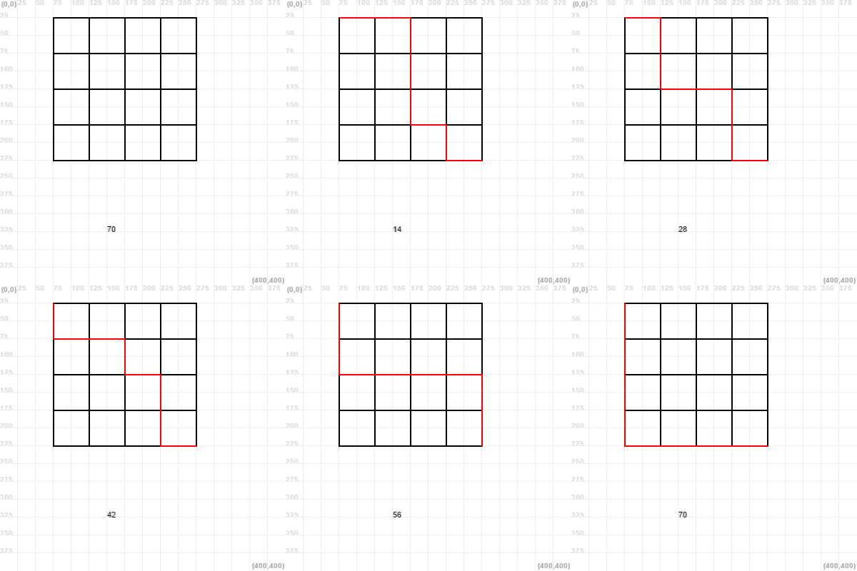
Can you make a recursive program to draw all possible paths from the Top-Left corner to the Bottom-Right one?
Here you have an image with all the possible paths for the 4x4 grid!

